A streaming service ran an A/B test on a new recommendation engine and wanted to know whether to roll it out. The naive comparison said yes. The careful comparison agreed and raised the estimate, because the treatment group happened to be older than the control group and age is the single strongest negative predictor of hours watched in the dataset. The new engine was carrying a handicap the headline number did not show.
The test data covered 1,000 users, 880 on the incumbent recommender and 120 on the new one, with hours watched over the test period as the engagement metric. Alongside it sat age, a social engagement score, months since signup, gender and a four-level demographic code.
A Welch two-sample t-test on hours watched put Group B at 4.81 hours against Group A’s 4.34, a gap of 0.47 hours significant at p = 0.0003. That is where a lot of A/B analyses stop. The problem is that random assignment had not delivered balanced groups: a t-test on age alone showed Group B averaging 38.9 years against Group A’s 36.2, a difference of 2.8 years significant at p = 0.005. Every additional year of age costs about 0.065 hours watched. Group B was starting roughly 0.18 hours behind before the engine did anything.
Regressing hours watched on age, social engagement, tenure, group, gender and demographic recovered a group effect of +0.64 hours, larger than the raw 0.47-hour gap, because the model gives the new engine credit for the age it was working against. Age came in at -0.065 hours per year and social engagement at +0.095 hours per point, both overwhelmingly significant. Tenure, gender and demographic did nothing.
The finding that changed the rollout advice came from adding interaction terms. Group crossed with age was flat and not significant, so the engine works about as well on older users as younger ones. Group crossed with social engagement was significant at p = 0.009, with a coefficient of +0.091. For a user scoring zero on social engagement the new engine is worth almost nothing measurable. For a user scoring ten it is worth close to a full extra hour on top of the base effect. The lift is real and it is concentrated.
So the recommendation was not simply “ship it”. It was ship it, and expect the gain to show up first and most clearly in the socially engaged cohort, which is where production monitoring should be pointed.
In brief
- 1,000 users, 880 on the incumbent recommender (Group A) and 120 on the new one (Group B)
- Welch t-test on hours watched: Group A 4.34, Group B 4.81, t = -3.67, p = 0.000332
- Shapiro-Wilk on hours watched returned W = 0.998, p = 0.25, so parametric methods were appropriate
- Age imbalance: Group A 36.15 years, Group B 38.94 years, p = 0.005, with Group B the older of the two
- Initial regression: age -0.065 hours per year, social engagement +0.095 hours per point, group +0.643 hours, all at p < 0.001
- Adjusting for age raised the estimated group effect from the raw 0.47 hours to 0.64 hours
- Group by social-engagement interaction: +0.091, p = 0.00927; group by age interaction: -0.0035, p = 0.72
- Adjusted model R² = 0.405 on five terms, F = 135.1 on 5 and 994 degrees of freedom
- Social engagement itself was balanced between groups (p = 0.20), so the interaction is not an artefact of assignment
The report as submitted
1. Introduction
The service introduced a new recommendation engine and ran a controlled test to find out whether it increased the time users spend watching content. Users on the previous engine formed the control group, Group A. Users on the new engine formed the treatment group, Group B. The metric of interest was hours watched per user over the test window.
The decision the analysis had to support was a rollout decision: whether to move the whole user base onto the new engine. That requires more than a difference in means. It requires confidence that the difference is attributable to the engine rather than to whatever else happens to differ between the two groups.
2. The data
The dataset held 1,000 observations across eight variables.
| Variable | Type | Range |
|---|---|---|
| group | Categorical | A (control, n = 880), B (treatment, n = 120) |
| age | Numeric | 18 to 55, mean 36.49 |
| social_metric | Numeric | 0 to 10, mean 4.91 |
| hours_watched | Numeric | 0.50 to 8.30, mean 4.39 |
| time_since_signup | Numeric | 0 to 24 months, mean 11.97 |
| demographic | Categorical | Four levels |
| gender | Categorical | F, M |
| date | Character | Test-window date |
The social metric is a composite score for a user’s engagement with the platform’s social features, on a zero to ten scale.
3. Preprocessing and the normality check
Dates were parsed, rows missing hours_watched were dropped, and group, gender and demographic were converted to factors so they would be handled as categories rather than numbers in the models.
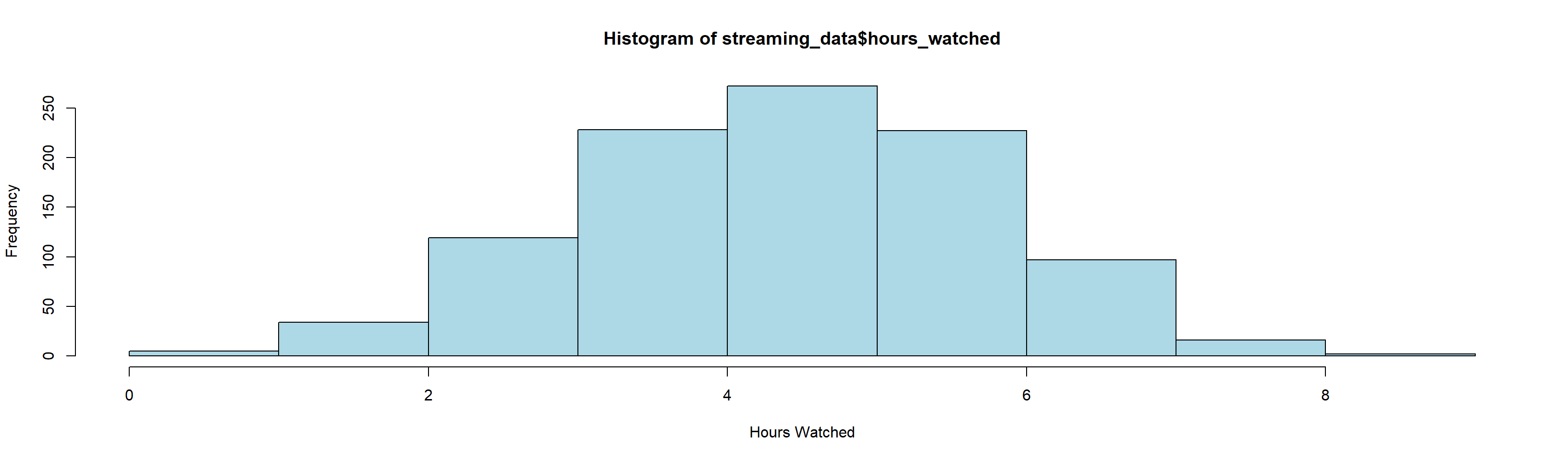
The parametric methods planned for the analysis assume an approximately normal dependent variable, so that was checked rather than assumed.
shapiro.test(streaming_data$hours_watched)
# W = 0.99792, p-value = 0.2495
The Shapiro-Wilk test does not reject normality, so t-tests and linear regression are appropriate here.
4. The headline comparison
t.test(hours_watched ~ group, data = streaming_data)t = -3.672, df = 153.01, p-value = 0.000332
95 percent confidence interval: -0.7302 to -0.2193
mean in group A: 4.336 mean in group B: 4.811Users on the new engine watched 0.47 hours more on average, and the difference is unlikely to be chance. This is a genuine signal and an insufficient basis for a rollout, because it says nothing about whether the two groups were comparable to begin with.
5. Initial regression
Hours watched was regressed on all six candidate predictors.
lm_model <- lm(hours_watched ~ age + social_metric + time_since_signup +
group + gender + demographic, data = streaming_data)| Term | Estimate | Std. error | t | p |
|---|---|---|---|---|
| (Intercept) | 6.2992 | 0.1966 | 32.04 | < 2e-16 |
| age | -0.0652 | 0.0060 | -10.83 | < 2e-16 |
| social_metric | 0.0953 | 0.0110 | 8.70 | < 2e-16 |
| time_since_signup | 0.0035 | 0.0045 | 0.77 | 0.441 |
| groupB | 0.6428 | 0.1022 | 6.29 | 4.85e-10 |
| genderM | -0.1829 | 0.1426 | -1.28 | 0.200 |
| demographic2 | 0.1452 | 0.1397 | 1.04 | 0.299 |
| demographic3 | -0.2318 | 0.1506 | -1.54 | 0.124 |
Residual standard error 1.034 on 992 degrees of freedom. Multiple R² 0.4023, adjusted R² 0.3981. F = 95.37 on 7 and 992 degrees of freedom.
Three things are worth pulling out.
Age is the dominant predictor. Each additional year is associated with 0.065 fewer hours watched, so the gap between an 18-year-old and a 55-year-old is roughly 2.4 hours, well over half the mean.
The group coefficient of 0.643 is larger than the 0.475 raw difference from the t-test. That is the adjustment working: once age is held constant, the new engine looks better than the unadjusted comparison suggested.
The fourth demographic level returned NA because of a singularity, meaning it was linearly dependent on the other terms in the model and could not be estimated separately. Since none of the demographic levels approached significance, this was noted and the variable dropped rather than respecified.
An ANOVA over the same specification agreed with the regression on which terms matter: age (F = 544.6), social engagement (F = 79.7) and group (F = 40.7) all significant, with tenure, gender and demographic all non-significant.
6. The age imbalance
The regression made the imbalance worth testing directly.
t.test(age ~ group, data = streaming_data)
# t = -2.8185, df = 157.95, p-value = 0.005443
# mean in group A: 36.15    mean in group B: 38.94

t.test(social_metric ~ group, data = streaming_data)
# t = -1.2752, df = 157.33, p-value = 0.2041
# mean in group A: 4.87     mean in group B: 5.23
Group B was older than Group A by 2.79 years, and the difference is significant. Group B also scored marginally higher on social engagement, but that difference is not significant and can be treated as noise.
The direction of the age imbalance matters. Age depresses hours watched, and the treatment group is the older one, so the imbalance works against the new engine rather than for it. An analyst who noticed the imbalance but not its direction might have assumed the raw result was inflated. It was deflated.
7. Adjusted regression with interaction terms
The final model kept the three predictors that carried weight and added interactions between group and each of the two continuous predictors, to test whether the engine’s effect varies by user type.
$$ \text{Hours} = \beta_0 + \beta_1\text{Age} + \beta_2\text{Social} + \beta_3\text{Group} + \beta_4(\text{Age} \times \text{Group}) + \beta_5(\text{Social} \times \text{Group}) $$
final_model <- lm(hours_watched ~ age + social_metric + group +
age:group + social_metric:group, data = streaming_data)| Term | Estimate | Std. error | t | p |
|---|---|---|---|---|
| (Intercept) | 6.5359 | 0.1364 | 47.92 | < 2e-16 |
| age | -0.0723 | 0.0032 | -22.28 | < 2e-16 |
| social_metric | 0.0849 | 0.0116 | 7.35 | 4.28e-13 |
| groupB | 0.3048 | 0.4307 | 0.71 | 0.479 |
| age:groupB | -0.0035 | 0.0099 | -0.35 | 0.724 |
| social_metric:groupB | 0.0914 | 0.0351 | 2.61 | 0.00927 |
Residual standard error 1.031 on 994 degrees of freedom. Multiple R² 0.4047, adjusted R² 0.4017. F = 135.1 on 5 and 994 degrees of freedom.
The ANOVA on the same specification confirms it: the group by social-engagement interaction is significant (F = 6.80, p = 0.00927) and the group by age interaction is not (F = 0.073, p = 0.787).
The groupB main effect is no longer significant on its own, which is expected once interactions are in the model. It now represents the engine’s effect for a hypothetical user with a social metric of zero, and at that end of the scale the engine does very little. The engine’s value is in the interaction, not the intercept shift.
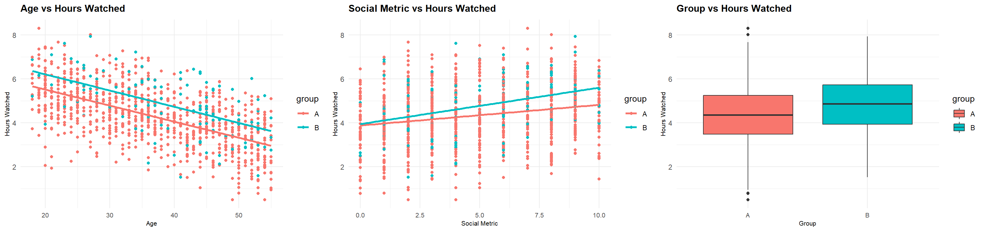
The middle panel is the finding. Both groups gain hours as social engagement rises, and Group B’s line is steeper. The left panel is the finding that did not hold: the two age slopes look slightly different by eye, but the interaction term says that apparent difference is within noise.
8. Discussion
What the analysis shows. The new recommendation engine increases hours watched. The effect survives adjustment for the age imbalance in the assignment, and adjusting for that imbalance increases rather than decreases the estimate. The size of the effect depends on how socially engaged the user already is, with the gain widening by about 0.09 hours for every point on the ten-point social scale.
Strengths. The imbalance in the test groups was found and corrected rather than reported as a caveat. Interaction terms were used to test a specific hypothesis about where the effect lives instead of being added speculatively. The distributional assumption behind the tests was checked before the tests were run.
Limitations. Hours watched is the only engagement measure considered. Content variety, session frequency, completion rates and return visits are all plausible measures the engine might move in different directions, and none of them are in this dataset. The treatment group is small at 120 users, which is why the interaction estimate carries a standard error a third the size of the coefficient itself. The test window is short and says nothing about whether the lift persists or decays as novelty wears off.
The analysis also cannot distinguish between two explanations of the interaction. The engine may genuinely serve socially engaged users better, or socially engaged users may simply have more headroom to increase their viewing. Separating those would need a design that varies social engagement rather than observing it.
Next steps. Extend the measurement set beyond hours watched. Rerun with a larger treatment arm to tighten the interaction estimate. Track the socially engaged cohort separately through the rollout, since that is where the model predicts the effect will be visible earliest.
9. Conclusion
Roll out the new engine. The evidence for an average effect is strong, and it holds after controlling for the one variable that was meaningfully unbalanced between the test groups. Expect the gain to be uneven across the user base, and watch the socially engaged segment first, because that is where the model says the difference will show up before anywhere else.
References
Wickham, H & Chang, W 2023, ggplot2: elegant graphics for data analysis, viewed 6 October 2024, https://ggplot2.tidyverse.org.
Wickham, H, François, R, Henry, L & Müller, K 2023, dplyr: a grammar of data manipulation, viewed 6 October 2024, https://dplyr.tidyverse.org.
Xie, Y 2023, knitr: a general-purpose package for dynamic report generation in R, viewed 6 October 2024, https://yihui.org/knitr/.
Auguie, B 2017, gridExtra: miscellaneous functions for “grid” graphics, viewed 6 October 2024, https://cran.r-project.org/web/packages/gridExtra/index.html.
Welch, BL 1947, ‘The generalization of “Student’s” problem when several different population variances are involved’, Biometrika, vol. 34, no. 1-2, pp. 28-35.
University of California, Los Angeles, n.d., Linear regression in R, viewed 6 October 2024, https://stats.idre.ucla.edu/r/dae/linear-regression-in-r/.
CRAN, n.d., ANOVA (analysis of variance) in R, viewed 6 October 2024, https://cran.r-project.org/web/packages/easyanova/index.html.
RMIT University 2024, Streaming engagement dataset, provided for educational purposes, viewed 6 October 2024.