A spam filter that is 94.4% accurate sounds finished. This one caught 60% of the spam. Both statements describe the same model on the same test set, and the gap between them is the entire point of the exercise: on imbalanced data, accuracy measures how well you predict the majority class, and it will happily report success while the thing you actually care about goes uncaught.
The setup was a mobile network operator wanting to replace number blacklisting, which spammers defeat by rotating numbers, with a classifier that reads the message instead. 5,351 SMS messages, 704 of them spam. That is 13.2% positives, which is imbalanced enough to break the default metric without looking obviously broken.
The arithmetic is unforgiving. A model that predicts “not spam” for every single message scores 86.8% accuracy while providing no filtering whatsoever. Any real model has to beat that baseline, and beating it by a few points says almost nothing about whether the model is useful.
Underneath that sat the ordinary text problem: raw SMS is short, noisy, full of abbreviations and non-words, and has to become a numeric matrix before any classifier can touch it. The cleaning decisions made there constrain everything downstream.
Four models were trained, two families each run once on the natural class distribution and once on data rebalanced with SMOTE. The headline result is that the model with the best accuracy and the model with the best balanced accuracy are not the same model, and only one of the two columns is answering the question a spam filter exists to answer.
Rebalancing the training data moved spam recall from 60% to 87% for one of those families while accuracy moved by two tenths of a point in the wrong direction. Read the accuracy column and nothing happened. Read the confusion matrices and forty spam messages that would have reached the inbox no longer do, at the price of forty-two legitimate messages that now sit in a spam folder. That is a real trade with a real cost on both sides, and it is invisible in the metric most people would report.
The second finding is that rebalancing is not a general-purpose fix. The same treatment that added eleven points of balanced accuracy to the nearest-neighbour model took nearly five points off the decision tree.
In brief
- 5,351 SMS messages, 704 spam (13.2%); the all-negative baseline scores 86.8% accuracy while filtering nothing
- Pipeline: NLTK tokenisation and stopword removal, bag-of-words vectorisation to 8,792 features, grid search per model
- SMOTE applied to the training split only (3,727 of 7,454 samples positive); test set held at its natural imbalance of 151 spam in 1,071 messages
- Best accuracy and best balanced accuracy identify different models: decision tree at 95.33% accuracy, KNN with SMOTE at 91.09% balanced accuracy
- Rebalancing raised spam recall from 60.3% (91 of 151) to 86.8% (131 of 151), at the cost of 42 false positives, while accuracy moved 0.19 points
- SMOTE improved KNN by 11 points of balanced accuracy and degraded the decision tree by 4.7, so it was reported as method-dependent rather than as a default
- Training completed in under 2 ms and prediction in under 0.3 ms per sample, ruling compute out as a selection criterion
The analysis in full
This work was submitted as a Jupyter notebook and a slide deck rather than a written report, so what follows is reconstructed from the notebook’s code, printed outputs and figures, and from the deck’s framing. Where the analysis has a flaw, it is reported here rather than smoothed over.
1. The dataset
The source file held 5,351 rows across four columns, two of which were artefacts: an unnamed integer index and a second unnamed column with 49 non-null values and no defined meaning. The two columns that mattered were sms, the raw message text, and spam, a boolean.
Splitting on that boolean gave 704 spam messages against 4,647 legitimate ones, a spam proportion of 13.16%.
That ratio is the whole reason the project needs a second metric. A classifier that never predicts spam is right 86.8% of the time. The distance between 86.8% and the 94.4% the first model scored is 7.6 points, and it is not obvious from the accuracy figure alone how much of that gap represents useful filtering.
2. Cleaning and tokenisation
Each message was lowercased, stripped of punctuation via a character translation table, tokenised with NLTK’s word_tokenize, and filtered against the NLTK English stopword list.
Short messages make this step consequential in a way that long documents do not. A 200-word email survives aggressive cleaning; a 12-word SMS can lose most of its signal. Removing stopwords from “call now to claim your free prize” leaves four tokens carrying the entire classification.
3. Vectorisation
The cleaned token lists were rejoined into strings and passed through CountVectorizer with English stopwords excluded, producing a document-term matrix of 5,351 rows by 8,792 features. Each cell is a raw term count.
This is bag of words, not TF-IDF. Nothing downweights terms that appear across the whole corpus, so common words that survived both stopword passes carry the same per-occurrence weight as rare discriminating ones. For spam specifically, TF-IDF would have been the better instinct, because the words that separate the classes are exactly the ones that appear constantly in one class and almost never in the other, and that is the contrast TF-IDF is built to amplify. The decision to use raw counts is the clearest thing I would change if I ran this again.
Stopwords were also removed twice, once by NLTK during tokenisation and again by the vectoriser. Harmless, but redundant.
4. Split and hyperparameter search
An 80/20 train-test split with a fixed random seed gave 4,280 training and 1,071 test messages, with 151 spam messages in the test set. The test set was never rebalanced. Rebalancing it would measure performance in a world that does not exist.
Two model families were searched with GridSearchCV, scored on accuracy:
| Model | Search space | Selected |
|---|---|---|
| K-nearest neighbours | n_neighbors in 1, 3, 5, 9, 11; p in 1, 2 | n_neighbors=1, p=2 |
| Decision tree | max_depth in 2, 3, 5, 10, 20; min_samples_leaf in 5, 10, 20, 50, 100; min_samples_split in 2, 3, 5 | max_depth=20, min_samples_leaf=5, gini |
Both searches went to the edge of their grid, and both selections are worth flagging. n_neighbors=1 means the classifier assigns each test message the label of its single closest training message, which is closer to lookup than to generalisation. max_depth=20 was the deepest value offered, so the true optimum may lie outside the grid. Both are consequences of scoring the search on accuracy, which on this data rewards caution about predicting the minority class.
SMOTE was then applied to the training split only, synthesising minority examples until the training set reached 7,454 samples with exactly 3,727 positives, a 50-50 split. Each model family was refit on that.
5. Results
| Model | Accuracy | Balanced accuracy | Spam recall | Spam precision |
|---|---|---|---|---|
| KNN | 94.40% | 80.13% | 60.3% | 100% |
| KNN + SMOTE | 94.21% | 91.09% | 86.8% | 75.7% |
| Decision tree | 95.33% | 85.93% | 72.8% | 92.4% |
| Decision tree + SMOTE | 93.37% | 81.20% | 64.2% | 85.1% |
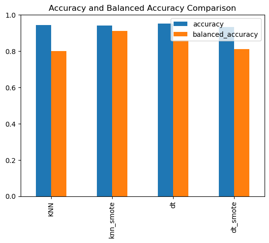
Read the accuracy column alone and the decision tree wins. Read the balanced accuracy column and it comes third. The accuracy column spans two points across all four models; the balanced accuracy column spans eleven. One of those columns is discriminating between the models and the other is not.
6. The confusion matrices
The disagreement becomes concrete once you count messages instead of percentages.
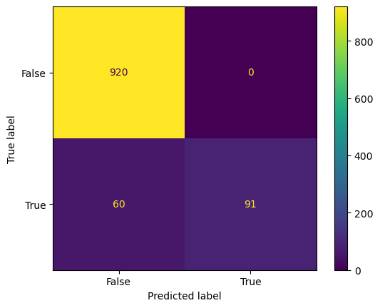
Plain KNN: zero false positives, which looks excellent, and 60 spam messages out of 151 sent straight to the inbox. Perfect precision at 60.3% recall. The model achieved its 94.4% by being cautious in exactly the direction that makes it useless.
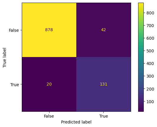
The same model on SMOTE-rebalanced data: spam caught goes from 91 to 131, so recall moves from 60.3% to 86.8%. The cost is 42 false positives where there were none. Accuracy moves from 94.40% to 94.21%, which is to say it does not move at all, while balanced accuracy climbs eleven points.
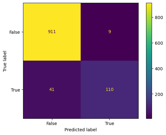
The decision tree sits between them: 110 of 151 spam caught at 9 false positives. That is the best raw accuracy of the four and a genuinely reasonable filter, though it still lets 41 spam messages through.
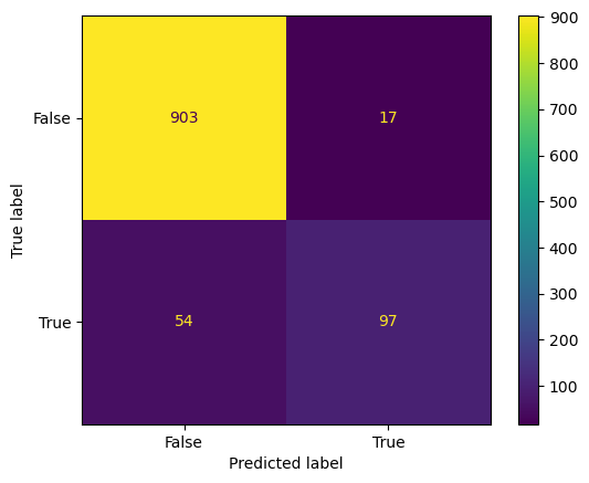
The decision tree on rebalanced data gets worse on both sides: fewer spam caught (97 against 110) and more false positives (17 against 9).
7. The trade is a product decision
Forty-two legitimate messages in the spam folder against forty fewer spam messages in the inbox is a question about which mistake annoys the user more, and no metric answers it on the analyst’s behalf. For a mobile operator the asymmetry is real: a missed spam is an irritation, a filtered appointment reminder or two-factor code is a support call. The right answer depends on whether the filter hides messages or flags them, and that is a design decision upstream of the model.
What the analysis can say is that the trade is available and roughly linear in this region, and that choosing on accuracy alone hides it entirely.
8. SMOTE is not a general-purpose fix
It helped KNN substantially, adding 11 points of balanced accuracy, and it made the decision tree worse, dropping balanced accuracy from 85.93% to 81.20%.
The likely reason is the interaction between how SMOTE generates samples and how each model draws boundaries. SMOTE interpolates between existing minority points. In a sparse, high-dimensional count matrix, the interpolated points sit in regions where no real message lives. A distance-based model tolerates that reasonably well, because the synthetic points still pull the local neighbourhood in the right direction. A tree splitting on axis-aligned thresholds can end up carving boundaries that fit the interpolations rather than the class, and a depth-20 tree with a five-sample leaf minimum has plenty of capacity to do exactly that.
The general form of the conclusion is that rebalancing is a method-dependent intervention that has to be measured per model, not a preprocessing step applied by default.
9. Compute cost
All four models trained in under two milliseconds and predicted in well under a millisecond per sample. Nothing here was decided on compute, which is worth recording precisely because compute is often the tiebreaker, and here it was not.
One caveat on those numbers. The evaluation helper takes a cross-validation results object as an argument, and for the two decision tree runs the KNN search results were passed in by mistake. The timing figures reported for the decision tree are therefore KNN’s timings, not the tree’s. The accuracy and balanced accuracy figures are computed from the actual predictions and are unaffected. The conclusion that compute is not a differentiator survives, because all four models are trivially cheap at this data size, but the specific per-model timings for the decision tree should not be quoted.
10. Recommendation and limitations
KNN with SMOTE is the model to deploy, on the basis that it catches 87% of spam and that the false positive cost is manageable and tunable. The decision tree is the better choice if false positives are treated as much more expensive than missed spam, which is a defensible position for a carrier and would need to be stated as a policy rather than discovered from a metric.
The limitations are worth being direct about. The vectoriser should have been TF-IDF. n_neighbors=1 means the deployed model is effectively memorising the training set, which will degrade as spam vocabulary drifts and gives no smoothing against a single mislabelled training example. The grid search was scored on accuracy, the exact metric this project argues against, so the hyperparameters were chosen by the wrong criterion even where the models were then judged by the right one. And the whole evaluation rests on one 80/20 split of a corpus of 5,351 messages, with 151 spam in the test set, so differences of a percentage point or two between models are not meaningful.
None of that changes the finding, which is about the metric rather than the model: on data at 13% positives, accuracy is not a measure of whether the filter works.