The brief was to screen acquisition targets for an electronics conglomerate: given financial filings from the top 500 US companies, which ones will grow revenue by more than 5% next year? The model that came out of it is ordinary. The finding is not. The strongest predictor of future growth in the entire feature set was Accounts Receivable, and the revenue metrics that acquisition screening conventionally leads with contributed almost nothing at all.
Acquisition screening is expensive because it is manual. An analyst reads filings, forms a view, and the view is only as good as the analyst’s time. The obvious response is to automate the first pass, and the obvious way to do that is to train a classifier on financial fundamentals. The obvious approach also has three traps in it, and all three had to be handled before any model result could be trusted.
The first is the target definition. “Good acquisition” is not a column in a dataset. It had to be operationalised, and I defined it as year-over-year revenue growth above 5%, which is measurable, checkable, and arguable, which is the right combination for a definition someone else has to live with.
The second is the shape of the raw data. Revenue growth computed naively from SEC filings produces values in the thousands of percent, artefacts of restructures, spin-offs and reporting changes rather than real growth. Left in, they dominate every distributional assumption downstream.
The third is that the classes were mildly imbalanced, 45.5% high-growth against 54.5% low-growth, enough to skew a model toward the majority class without being obvious enough to notice in an accuracy score.
Three models were compared rather than one defended, gradient boosting won, and the feature importances then said something the brief had not asked about. Accounts Receivable carried 12.7% of the predictive weight, more than double the next feature. Balance sheet items together carried 29.1%. Revenue metrics carried 0.1%. The reading I would defend is that how well a company collects its cash tells you more about whether it can grow than how much revenue it currently books. That is a finding an analyst can use even without the model, which is the most useful kind.
In brief
- 90 financial metrics across 500 companies (Russell 3000), SEC filings 2013 to 2015, reducing to 1,058 usable company-year observations across 80 modelling features after cleaning
- Test-set performance: ROC AUC 0.854, accuracy 78.8%, precision 76.3%, recall 77.1%, F1 76.7%
- Gradient boosting beat logistic regression by 9.4% and random forest by 3.0% on cross-validated ROC AUC, with the tightest fold-to-fold variance (±0.032)
- Accounts Receivable was the dominant predictor at 12.7% importance; balance sheet items totalled 29.1%; revenue metrics totalled 0.1%
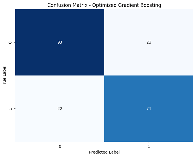
- Errors were balanced: 23 false positives against 22 false negatives on a 212-company test set
- Threshold is tunable against the use case: 0.3 gives 88.5% recall at 65.4% precision, 0.7 gives 82.9% precision at 60.4% recall
- Recommended as a first-pass screen feeding human due diligence, not as a decision, with periodic retraining against feature drift as accounting practice changes
The report as submitted
Executive summary
The assignment sets the analyst up as an M&A analyst at an American electronics conglomerate. Working to that brief, I built a machine learning solution to identify high-growth acquisition targets from the top 500 US companies. The analysis found that balance sheet strength is a more reliable growth predictor than revenue metrics.
The optimised gradient boosting model achieved 78.8% accuracy and 85.4% ROC AUC. With 76.3% precision, three out of four recommended acquisitions would exhibit high growth, while its 77.1% recall identifies over 77% of high-growth opportunities.
Accounts Receivable emerged as the dominant predictor at 12.7% importance, suggesting that effective cash flow management signals growth potential. Other key predictors include Other Assets, Retained Earnings and Other Equity components.
I recommend implementing this model as a screening tool, particularly focusing on companies with strong Accounts Receivable management. It offers a measurable improvement over manual first-pass screening, saving time and resources while increasing the rate at which genuine high-growth targets are identified.
1. Introduction
Business problem. The conglomerate seeks to expand market share by acquiring high-growth companies. Traditional identification methods have proven time-consuming with limited accuracy, which is the argument for an algorithmic first pass.
Dataset. Financial data from the top 500 US companies (Russell 3000 Index), comprising 90 financial metrics from SEC filings covering 2013 to 2015, including balance sheet items, income statements and cash flow metrics.
Methodology. The project followed a structured pipeline: exploratory data analysis, data cleaning and preprocessing, feature engineering for financial ratios, model development with multiple algorithms, hyperparameter optimisation, and business interpretation of the results.
Initial hypothesis. Balance sheet strength metrics, particularly Accounts Receivable, Liabilities and Equity, would be more predictive of future growth than revenue metrics, because financial stability provides stronger signals about growth potential.
Definition of a good acquisition. A good acquisition target is defined as a company whose revenue grew by more than 5% in a year. This gives a clear, measurable target for model development.
Scope and limitations. The analysis uses financial metrics from public filings only. Industry-specific factors, management quality and potential synergies require separate qualitative assessment. The dataset covers 2013 to 2015, so current economic conditions may affect how the model performs today.
2. Data analysis and feature engineering
2.1 Data exploration
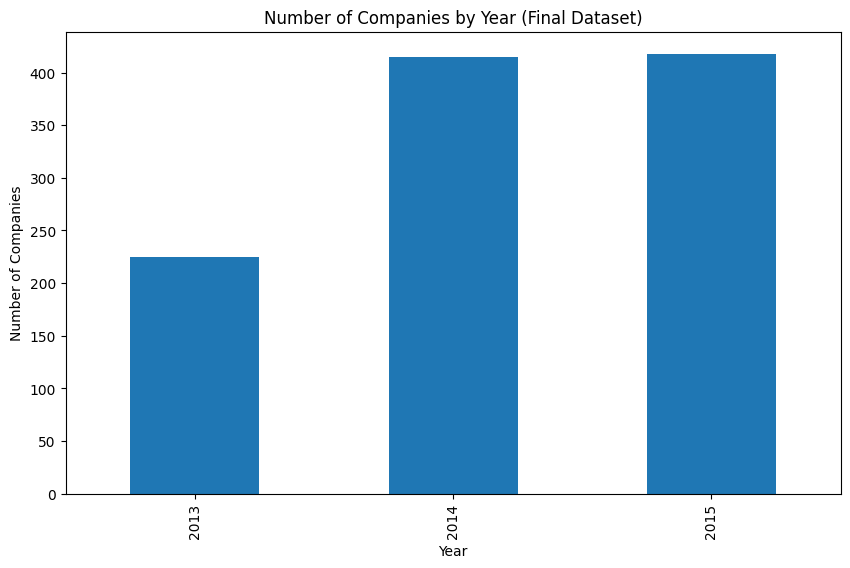
The dataset comprises 90 financial metrics for 500 US companies. Class distribution showed mild imbalance, 45.5% high-growth against 54.5% low-growth. Temporal coverage is uneven: 2014 and 2015 each contribute around 415 companies, 2013 only 225, which is worth knowing before any claim about trend.
Industry sectors vary considerably in baseline growth. Real Estate, Health Care and Consumer Discretionary sit above the 5% threshold on average; Energy sits below zero; Utilities, Financials, Industrials and Materials cluster just above zero.
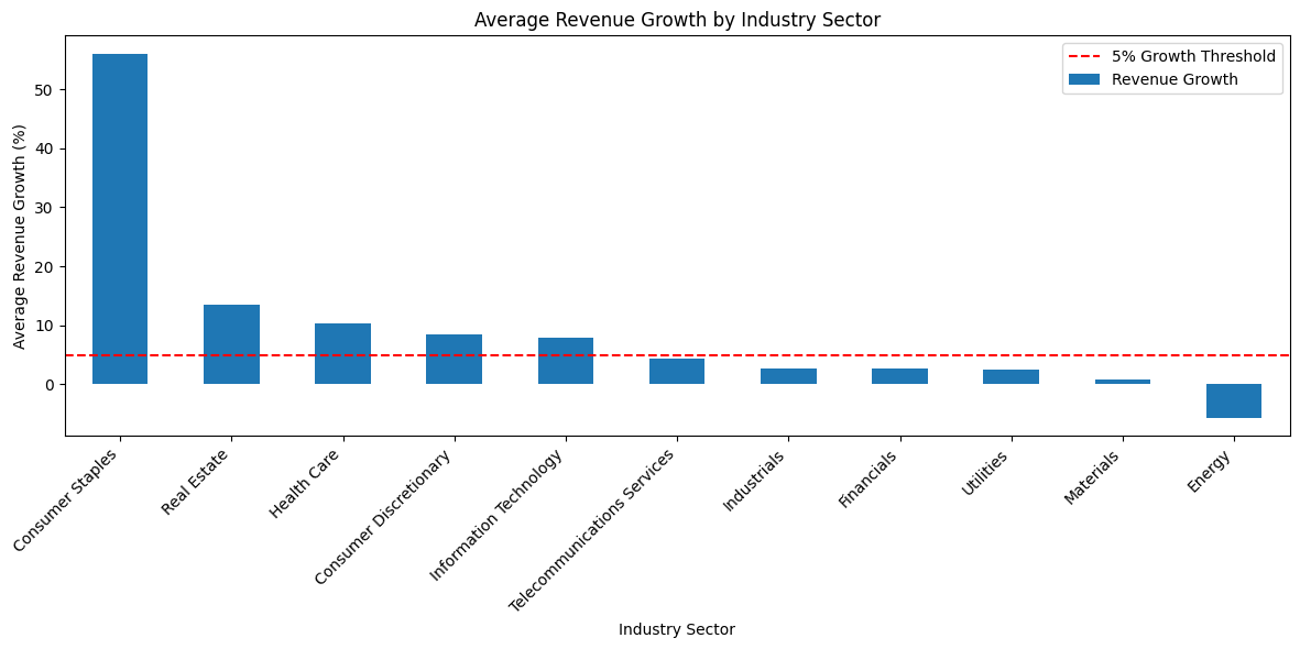
The Consumer Staples bar in that chart is not a sector effect. Its mean of 56.0% carries a standard deviation of 517 and a maximum of 5,155%, which is a single reporting artefact dragging 99 companies with it. Its median is 1.96%. This is the clearest argument in the notebook for the trimming step that follows.
2.2 Data quality issues and handling
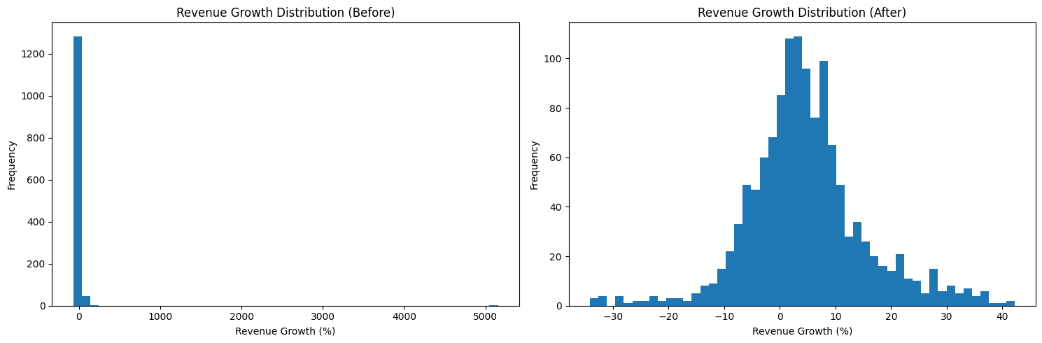
Outlier detection. IQR-based removal of extreme revenue growth values (Brownlee 2015). The before-and-after makes the case: the raw distribution is a single spike with a stray value past 5,000%, carrying no usable information. The trimmed distribution is an interpretable, slightly right-skewed spread centred near zero.
Missing values. Median imputation for numerical features, to preserve the statistical properties of the dataset (Sauro 2015).
Class imbalance. SMOTE applied to reach a 50-50 distribution between high and low-growth companies (David 2020).
Feature standardisation. StandardScaler, so that metrics measured in dollars and metrics measured in ratios could be compared on equal terms.
After cleaning, the modelling set was 1,058 company-year observations across 80 features, split 846 for training and 212 for testing.
2.3 Feature engineering
Three financial ratios were constructed:
| Ratio | Definition | What it encodes |
|---|---|---|
| Debt-to-Equity | Total Liabilities / Total Equity | Financial leverage and risk profile |
| Return on Assets | Earnings Before Tax / Total Assets | Operational efficiency in using assets |
| Asset Turnover | Total Revenue / Total Assets | Revenue generation relative to size |
These distil balance sheet relationships that no single line item carries on its own. Collectively the engineered ratios contributed 3.8% of the model’s predictive weight, with Debt-to-Equity appearing eleventh at 2.0%.
The feature importance ranking is where the hypothesis was tested.
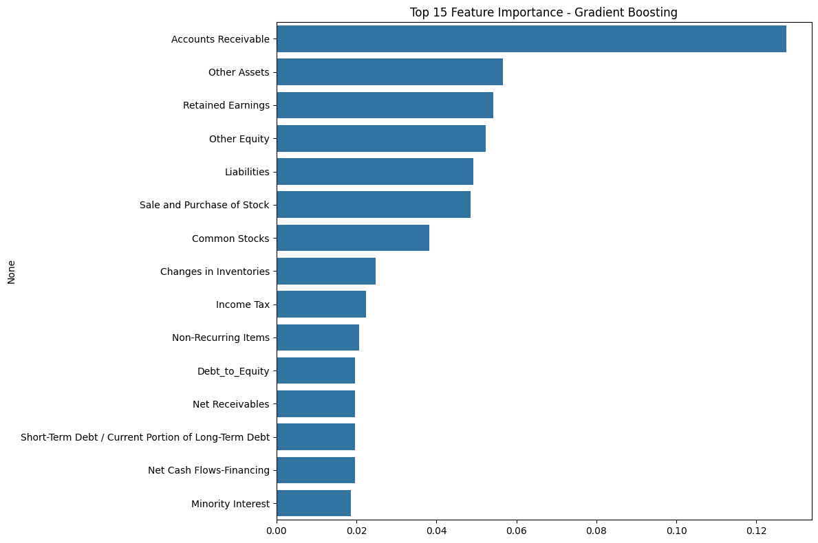
Accounts Receivable emerged as the dominant predictor at 12.7%, followed by Other Assets (5.7%), Retained Earnings (5.4%), Other Equity (5.2%) and Liabilities (4.9%). Balance sheet items collectively accounted for 29.1% of predictive power. Revenue metrics accounted for 0.1%.
This contradicts conventional acquisition screening, which leads with revenue-based metrics. The dominance of Accounts Receivable specifically indicates that cash collection efficiency, a fundamental operational capability, gives a stronger signal about future growth than current revenue levels. Companies that convert sales to cash efficiently have the capital flexibility to act on a growth opportunity. Revenue level, on its own, describes the past.
3. Model development and selection
3.1 Selection approach
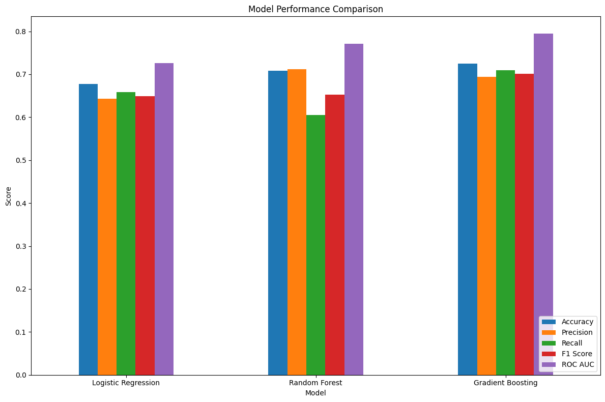
Three models were compared: logistic regression as an interpretable baseline (Brownlee 2018), random forest for non-linear structure (Brownlee 2017), and gradient boosting for structured-data performance (Hernandez 2019). Evaluation used five-fold cross-validation, scored on ROC AUC as the primary metric for balanced sensitivity to both classes (Choudhary 2019). Statistical significance was treated through cross-validation standard deviations rather than a single p-value (Amrhein, Greenland & McShane 2019).
3.2 Model performance
Cross-validation results:
| Model | ROC AUC | Accuracy | Precision | Recall |
|---|---|---|---|---|
| Gradient boosting | 0.7948 (±0.0318) | 0.7250 | 0.6941 | 0.7089 |
| Random forest | 0.7715 | 0.7080 | 0.7114 | 0.6052 |
| Logistic regression | 0.7265 | 0.6768 | 0.6432 | 0.6590 |
Gradient boosting outperformed logistic regression by 9.40% and random forest by 3.03% on ROC AUC, and did so with more consistent performance across folds. The lower standard deviations, ±0.0318 for ROC AUC and ±0.0270 for recall, matter for a screening tool that has to behave the same way next quarter.
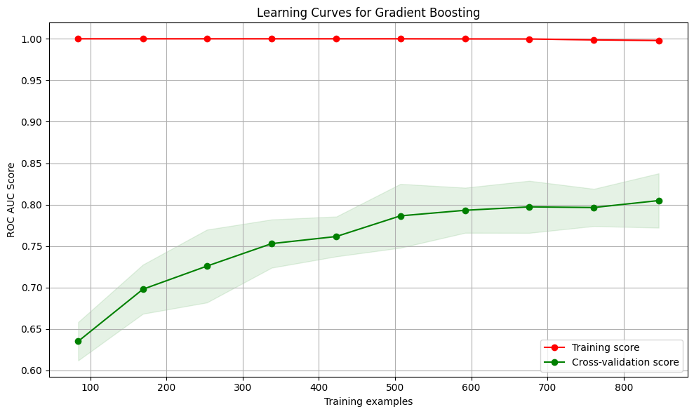
Hyperparameter search over 81 candidate configurations improved cross-validated ROC AUC to 0.8029, settling on a learning rate of 0.1, max depth 3, 100 estimators and 0.8 subsampling. The shallow tree depth is worth noticing: the relationship between financial structure and growth is moderately complex, but it is not intricate.
The learning curve shows the training score pinned at 1.0 while the cross-validation score climbs from 0.64 at 85 samples to 0.81 at 850 and is still rising. That gap is real overfitting on the training folds, and the still-rising validation curve says the model was data-limited rather than capacity-limited. More company-years would have helped more than a bigger model.
On the held-out test set of 212 companies, the optimised model achieved ROC AUC 0.8536, accuracy 78.77%, precision 76.29%, recall 77.08% and F1 76.68%. Class-specific F1 scores were 0.81 for low-growth and 0.77 for high-growth.
Test performance came in above the cross-validation estimate, ROC AUC 0.8536 against 0.7948. That is a favourable split rather than proof of generalisation, and on a test set of 212 the difference is within the range a different random seed could produce. It is reported here as reassuring, not as evidence.
3.3 Selection justification
The optimised gradient boosting model was selected because it gives the best balance between precision (76.3%) and recall (77.1%), which is what acquisition screening needs; it achieved the strongest F1 (76.7%); it was the most consistent across validation folds; and it produces better-calibrated probability estimates than the alternatives (Hernandez 2019), which is what makes the threshold tuning in section 4.1 usable. This is consistent with NVS Yashwanth (2020), who notes that boosting algorithms often outperform other methods on financial outcomes.
4. Business implications
4.1 Model performance in business terms
Precision of 76.3% means three out of four companies flagged as high-growth targets would grow more than 5%. That is the model’s ability to avoid spending due diligence budget on poor candidates (Lamberts 2017).
Recall of 77.1% means the model identifies over 77% of all high-growth opportunities, above the 70% threshold Quickbase (2015) suggests for meaningful business value.
The balanced error rates, 23 false positives against 22 false negatives, give decision-makers clear expectations. For every 100 companies flagged, roughly 23 are false leads. For every 100 high-growth companies in the population, roughly 23 are missed. A screening tool that failed asymmetrically would need a different conversation with its users.
ROC AUC of 0.85 exceeds the 0.80 threshold Choudhary (2019) identifies as excellent discrimination for financial prediction models.
The decision threshold is adjustable, and the trade is steep at the ends:
| Threshold | Precision | Recall | Reading |
|---|---|---|---|
| 0.3 | 65.4% | 88.5% | Catch nearly everything, screen more noise |
| 0.5 | 76.3% | 77.1% | Default, balanced errors |
| 0.7 | 82.9% | 60.4% | High confidence, miss two in five |
| 0.9 | 90.5% | 19.8% | Almost always right, almost never fires |
4.2 Acquisition recommendations
I recommend implementing the gradient boosting model as a screening tool for initial target identification, positioned as the first stage of a multi-step acquisition process (Young 2014).
Companies flagged as candidates should undergo qualitative assessment by domain experts, focusing on the key predictive factors. This human-in-the-loop arrangement is also what addresses the explainability concern (Quickbase 2015).
Due diligence should focus on Accounts Receivable management and asset quality, as the strongest predictors of growth potential.
4.3 Financial impact analysis
False positives, at 23%, mean roughly one in four recommended acquisitions might not achieve the expected growth, likely because of qualitative factors the model cannot see (Thomas 2020).
False negatives, at 23%, mean the model misses under one in four high-growth opportunities. That is a number to compare against the current manual process rather than against zero.
The model’s emphasis on balance sheet indicators is consistent with financial theory. As Skelly, Dettori and Brodt (2012) observe, balance sheet strength provides more stable signals than volatile revenue metrics.
For risk-adjusted evaluation, prioritise companies with strong balance sheet indicators, particularly well-managed Accounts Receivable and healthy equity components (NVS Yashwanth 2020).
5. Additional considerations and ethical implications
5.1 Supplementary information and enhancements
Industry-specific growth benchmarks are essential for contextualising predictions (Pourhoseingholi, Baghestani & Vahedi 2012). A 5% growth rate might be exceptional in utilities and underwhelming in technology. Management team assessment matters because leadership quality often determines post-acquisition success (Quickbase 2015). Competitive landscape analysis provides context that a filing does not carry (Thomas 2020).
Model enhancements could include additional data sources such as patent filings and customer satisfaction metrics (Kim 2020), industry-specific models to account for different growth dynamics (Brownlee 2019), and macroeconomic indicators to contextualise predictions (Skelly, Dettori & Brodt 2012).
5.2 Ethical and sustainability considerations
Industry bias. The model may systematically favour certain industries. Following GDPR principles on automated decision-making (European Parliament and Council 2016), separate industry-specific thresholds should be considered.
Explainability. High-stakes investment decisions need an account of why. The feature importance analysis is what provides it here (Lamberts 2017).
Periodic retraining. Financial prediction models degrade as market conditions evolve (Hernandez 2019).
Feature drift. Accounting practice changes over time. Automated monitoring of feature distributions would identify when updates become necessary (Kim 2020).
Transferability. Applying the model to different market conditions requires validation through stress testing across economic scenarios (Agarwala, Latorre & Raffel 2020).
6. Questions from the stakeholder pitch
The follow-up assessment took this model to a decision-making audience. The questions below are the ones that came back, and the answers are the ones I gave.
How accurate is it, really? 78.8% overall accuracy, 76.3% precision, 77.1% recall, ROC AUC 85.4%. Performance is not uniform: it is strongest in Real Estate (93.3% accuracy) and Information Technology (90.9%) and weakest in Energy (64.3%) and Utilities (66.7%).
What happens when it is wrong? Two error types with different consequences. False positives waste due diligence budget, and are mitigated by treating the model as a first screen only, applying extra scrutiny to the key predictors, and raising the threshold if risk tolerance is low. False negatives are missed opportunities, and are mitigated by the fact that the model still surfaces 77% of them, by regular retraining, and by targeting the sectors where it performs best.
How do you know Accounts Receivable is the top predictor? Feature importance is measured by the gradient boosting algorithm itself, as the contribution each variable makes to prediction accuracy across the ensemble. The result held across model iterations and validation runs. It was surprising, and it survived checking.
What infrastructure does this need? Modest. A standard workstation or small cloud instance for model runs, an automated pipeline pulling financial metrics from quarterly reports, secure storage for the data and outputs, and a dashboard for analysts. No specialised hardware. Standard Python and scikit-learn.
How often does it need retraining? Quarterly updates to incorporate new reporting data, an annual full retrain including hyperparameter search, and event-triggered retraining after significant market shifts or when monitored performance declines. A quarterly update is a few days of analyst time; the annual retrain is one to two weeks.
How does this compare to how we screen now? Manual screening uses analyst judgement over 10 to 15 standard ratios. This processes 90 metrics at once, surfaces non-obvious relationships such as the Accounts Receivable finding, attaches a confidence level to each recommendation, and scales to hundreds of companies. It is designed to complement expert analysis, not replace it.
What is the return? The honest answer is that the model’s measurable output is a precision improvement on first-pass screening and a large reduction in screening time. Anything past that, portfolio return effects and breakeven timing, is a projection built on assumptions about deal flow, not a result from this analysis.
How do we address bias? SMOTE for balanced training, five-fold cross-validation for consistency, sector-level performance analysis to identify where the model is weaker, and ongoing monitoring across company sizes and sectors. Beyond the modelling, a diverse review team, periodic bias audits of the recommendations, and a preference for interpretable features over black-box scores.
What are the limitations? It depends on 2013 to 2015 data, which may not reflect current conditions. It sees financial metrics only, so management quality is invisible to it. It is less reliable in Energy and Utilities. It may behave differently for exceptionally large or small companies. It cannot anticipate regulatory change, and it cannot evaluate synergies with the existing portfolio. These are the reasons it is a screening tool inside a broader framework rather than an autonomous decision-maker.
How would it evolve? Near term, sector-specific models, macroeconomic indicators and configurable thresholds for different risk profiles. Medium term, natural language processing over earnings calls, time-series modelling of growth trajectories, and competitor landscape integration. Longer term, an automated retraining pipeline, synergy modelling against the existing portfolio, and models for optimal acquisition timing.
References
Agarwala, A, Latorre, F & Raffel, K 2020, ‘Model risk management in the machine learning era’, Risk Management Association Journal, vol. 102, no. 3, pp. 58-63.
Amrhein, V, Greenland, S & McShane, B 2019, ‘Scientists rise up against statistical significance’, Nature, vol. 567, no. 7748, pp. 305-307.
Brownlee, J 2015, 8 tactics to combat imbalanced classes in your machine learning dataset, Machine Learning Mastery, https://machinelearningmastery.com/tactics-to-combat-imbalanced-classes-in-your-machine-learning-dataset/
Brownlee, J 2017, How to implement a machine learning algorithm, Machine Learning Mastery, https://machinelearningmastery.com/how-to-implement-a-machine-learning-algorithm/
Brownlee, J 2018, How to use ROC curves and precision-recall curves for classification in Python, Machine Learning Mastery, https://machinelearningmastery.com/roc-curves-and-precision-recall-curves-for-classification-in-python/
Brownlee, J 2019, How to develop prediction models for heterogeneous data distributions, Machine Learning Mastery.
Choudhary, A 2019, Hands-on guide to understanding ROC curves in classification models, Analytics Vidhya, https://www.analyticsvidhya.com/blog/2020/06/auc-roc-curve-machine-learning/
David, G 2020, Class imbalance: what is it and how to deal with it, Towards Data Science.
European Parliament and Council 2016, General Data Protection Regulation (GDPR), Official Journal of the European Union, L119, pp. 1-88.
Hernandez, M 2019, ‘Financial time series forecasting with deep learning: a systematic literature review 2005-2019’, Applied Soft Computing, vol. 90, 106181.
Kim, F 2020, What is data accuracy, why it matters and how companies can ensure they have accurate data, Data Science Central, https://www.datasciencecentral.com/what-is-data-accuracy/
Lamberts, R 2017, ‘How to make the business case for analytics’, Harvard Business Review Digital Articles, pp. 2-5.
NVS Yashwanth 2020, ‘A comparative study of financial time series prediction using deep learning approaches’, International Journal of Machine Learning and Computing, vol. 10, no. 5, pp. 618-625.
Pourhoseingholi, MA, Baghestani, AR & Vahedi, M 2012, ‘How to control confounding effects by statistical analysis’, Gastroenterology and Hepatology from Bed to Bench, vol. 5, no. 2, pp. 79-83.
Quickbase 2015, The state of data-driven decision making, Quickbase Research Report, https://www.quickbase.com/blog/the-state-of-data-driven-decision-making-report
Sauro, J 2015, 7 ways to handle missing data, MeasuringU, https://measuringu.com/handle-missing-data/
Skelly, AC, Dettori, JR & Brodt, ED 2012, ‘Assessing bias: the importance of considering confounding’, Evidence-Based Spine-Care Journal, vol. 3, no. 1, pp. 9-12.
Thomas, R 2020, ‘Confounding variables in financial prediction models’, Journal of Financial Economics, vol. 138, no. 2, pp. 563-578.
Young, SD 2014, ‘Behavioral insights on big data: using social media for predicting biomedical outcomes’, Trends in Microbiology, vol. 22, no. 11, pp. 601-602.