The hardest part of statistical communication is not the calculation. It is the surrounding framing: which question is being answered, what the answer means for a decision-maker, and what the analysis has actually licensed you to conclude. This assignment ran five inference exercises against simulated data with that framing question in the foreground every time.
The exercises had nothing to do with each other on the surface. A flu vaccine trial. An exponential distribution sampled a thousand times over. A packaging redesign. A pair of paired t-tests at two sample sizes. Three supermarket promotional strategies. What tied them together was that each one produced a number, and each number had a decision hanging off it, and in three of the five cases the honest reading of the number was “this does not tell you what you were hoping it would tell you.”
The packaging test is the one worth keeping. A new design scored 8.2 for attractiveness against the incumbent’s 7.5, on twenty respondents. The one-tailed t-test returned t = 1.65 against a critical value of 1.73, p = 0.0579. That is not a significant result, and it is not “almost significant” either. It is a result that says the evidence available is not enough to justify a packaging overhaul, and that a larger study might resolve it in either direction. The recommendation written up for management was to hold, and to say plainly that increasing the sample size carries no guarantee of a different answer. If the real effect is small, a bigger study will confirm that it is small.
The promotional ANOVA is the same lesson in a different costume. Three strategies, six stores each, simulated with true means five and ten points apart and a standard deviation of thirty. F = 2.351, p = 0.129. Rerun with the standard deviation tightened to twenty-five: F = 2.31, p = 0.133. Neither test rejects. The temptation is to write “no strategy outperforms the others.” The accurate statement is narrower: at six stores per arm and that much store-to-store variance, this design could not have detected a difference of the size that was actually built into the data. The test did not fail to find an effect. It was never able to look.
The middle exercise is the counterweight, and the only one that produced a clean result. Draw from a distribution as lopsided as an exponential, average two draws at a time, and the lopsidedness survives. Average thirty at a time and it is gone. Nothing changes except the sample size.
In brief
- Five methods covered: binomial proportion confidence interval, exponential sampling and the central limit theorem, one-tailed t-test, paired t-test at two sample sizes, one-way ANOVA
- Placebo group: 69 of 100 did not contract flu, giving a 95% Wald interval of 59.94% to 78.06% for the true proportion
- Population projection at 40% vaccination uptake: approximately 22% of adults contract flu in the season
- Ten-year binomial: 7.02% chance a consistently vaccinated person contracts flu three or more times in a decade
- Exponential sample of n = 1,000 returned a mean of 10.22 and standard deviation of 10.49 against theoretical values of 10 and 10
- Packaging redesign: t = 1.65 against a critical value of 1.73, p = 0.0579, recommendation was to hold rather than invest
- Paired t-tests on bivariate normal data with correlation 0.8: p = 0.0279 at n = 10, p = 0.0019 at n = 30
- Promotional ANOVA: F = 2.351, p = 0.129 at SD 30, and F = 2.31, p = 0.133 at SD 25, neither rejecting the null
- Every result reproducible from a single R Markdown file with
set.seed(3229642)
The report as submitted
1. Flu vaccine efficacy ahead of the winter season
A two-arm trial of 100 vaccinated participants and 100 placebo participants was simulated with per-person infection probabilities of 0.10 and 0.30 respectively.
set.seed(3229642)
contract_flu_A <- rbinom(1, 100, 0.10)   # vaccinated
contract_flu_B <- rbinom(1, 100, 0.30) # placebo| Condition | Group A (vaccinated) | Group B (placebo) |
|---|---|---|
| Contracted the flu | 20 | 31 |
| Did not contract the flu | 80 | 69 |
| Total | 100 | 100 |
Probability a placebo recipient avoids the flu. 69 of the 100 placebo participants did not contract flu, so the point estimate is 69%. Roughly seven in ten people who received the placebo got through the winter without infection, which is worth stating explicitly because it sets the baseline the vaccine has to beat.
A 95% confidence interval for that proportion. The interval was computed as a normal approximation, using the standard error of a proportion and z = 1.96.
std_error <- sqrt((prob_no_flu_B * (1 - prob_no_flu_B)) / 100)
ci_lower  <- prob_no_flu_B - 1.96 * std_error
ci_upper  <- prob_no_flu_B + 1.96 * std_error
That gives 59.94% to 78.06%. In plain language: repeat this trial many times over and construct the same interval each time, and about 95 intervals in 100 will contain the true placebo survival rate. The interval is wide, which is what 100 participants buys you. Anyone quoting the 69% without the interval is quoting a number with nine points of slack on either side of it.
Projecting to the wider population. If 40% of adults are vaccinated and the two infection probabilities hold, the expected population infection rate is the weighted average of the two arms:
p_flu_total <- 0.40 * 0.10 + 0.60 * 0.30 # 0.22Approximately 22% of the adult population would contract flu across the season. This figure is entirely contingent on the assumed 40% uptake, and it uses the design probabilities of 0.10 and 0.30 rather than the observed trial rates of 20% and 31%. Substituting the observed rates would raise the projection. Either choice is defensible, but the assumption has to travel with the number.
Ten years of vaccination. For someone vaccinated every year for ten years, with an annual infection probability of 0.10, the chance of contracting flu in three or more of those years is a binomial tail:
1 - pbinom(2, size = 10, prob = 0.10) # 0.07027.02%, or about seven people in a hundred. Low, but not negligible, and worth knowing if the communication objective is to set expectations rather than to sell certainty.
2. The distribution of the sample mean
The second exercise is a demonstration of the central limit theorem built from scratch rather than asserted.
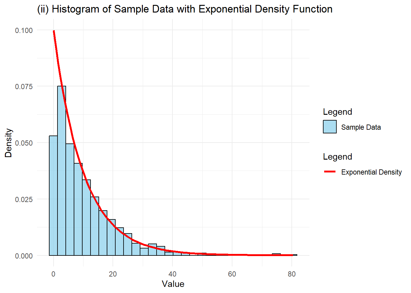
The source distribution. One thousand draws from an exponential distribution with rate 0.1, so a theoretical mean and standard deviation of 10 each.
sample_data <- rexp(1000, rate = 0.1)
mean(sample_data)   # 10.22
sd(sample_data)     # 10.49
Both sample estimates sit close to their theoretical values, which is what a sample of a thousand should deliver. The histogram, overlaid with the theoretical density, confirms the shape: heavily right-skewed, a mass of small values and a long thin tail.
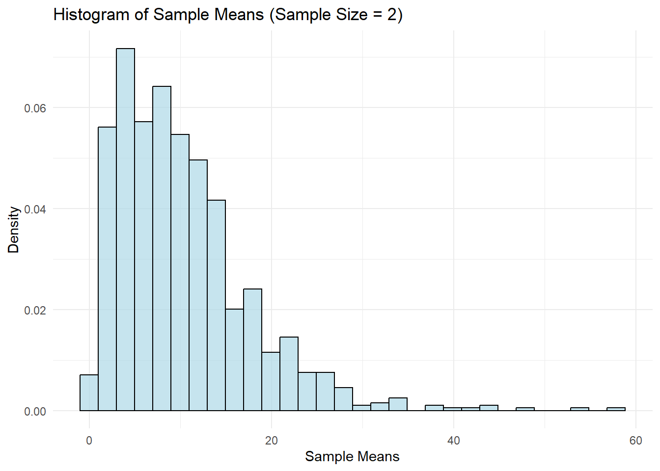
Sample means at n = 2. One thousand sample means, each the average of two draws.
sample_means_2 <- replicate(1000, mean(rexp(2, rate = 0.1)))The distribution of those means is still visibly right-skewed. Averaging two observations does very little to suppress the skew inherited from the source. The spread remains wide.
Sample means at n = 30. The same code with the sample size changed.
sample_means_30 <- replicate(1000, mean(rexp(30, rate = 0.1)))The result is approximately normal and much narrower, concentrated around the population mean of 10.
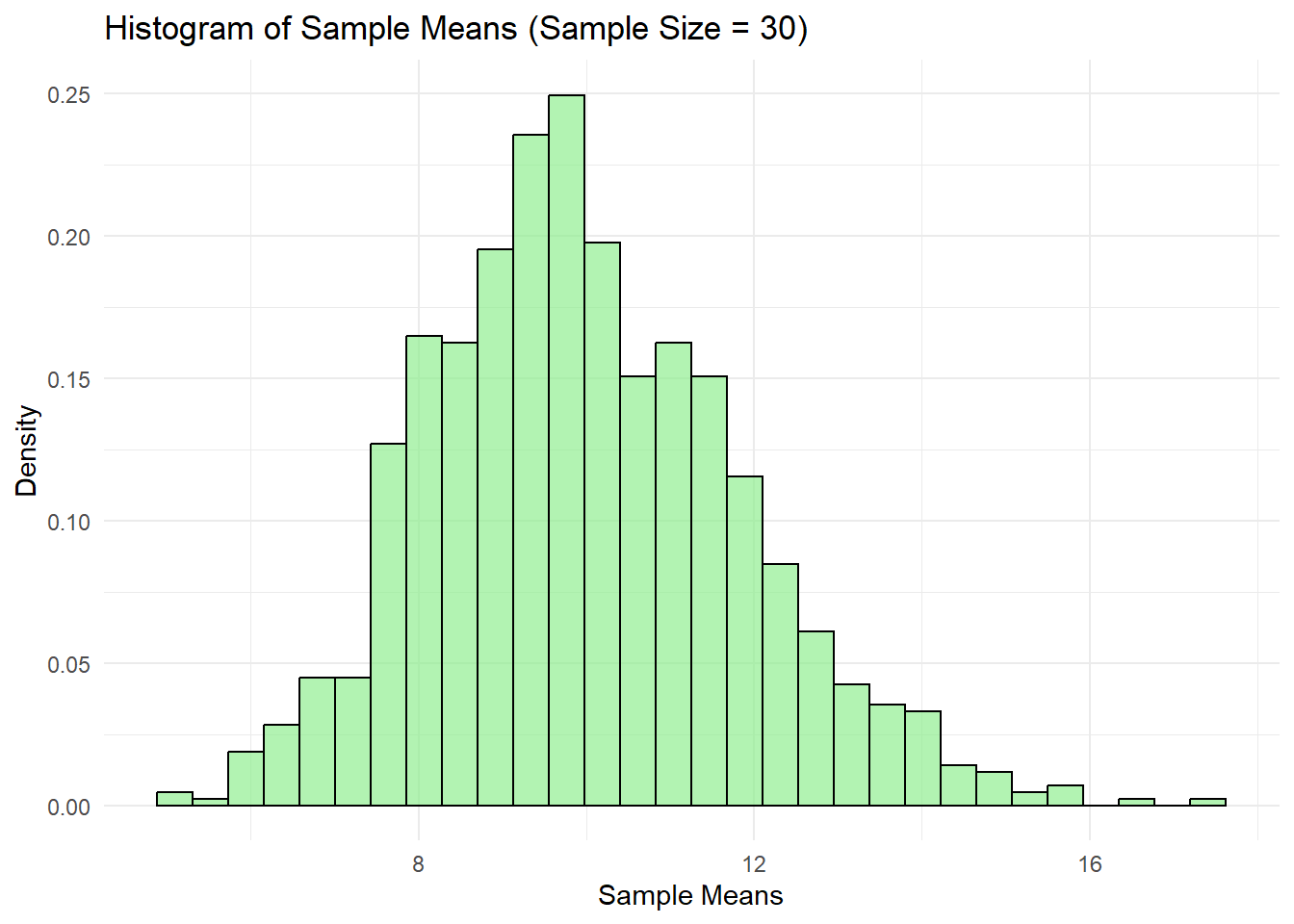
Three histograms, one changed parameter. The source distribution is as non-normal as a common distribution gets, and by n = 30 the sampling distribution of its mean is close enough to normal to use normal-theory tests on. That is the entire justification for the t-tests in the exercises that follow, and it is better shown than claimed.
3. A one-tailed t-test on packaging design
A survey of twenty respondents rated a proposed packaging design against the current one. Mean attractiveness moved from 7.5 to 8.2, with a standard deviation of the differences of 1.9.
t_value    <- (8.2 - 7.5) / (1.9 / sqrt(20))   # 1.65
t_critical <- qt(1 - 0.05, df = 19)            # 1.73
p_value    <- pt(t_value, 19, lower.tail = FALSE)  # 0.0579
The test statistic falls below the critical value and the p-value falls just outside the 5% threshold. The null hypothesis is not rejected.
The observed improvement is real in the sample and unproven in the population. There is roughly a 5.8% chance of seeing a difference this large if the two designs were genuinely equivalent, and the conventional threshold says that is not low enough to act on.
Three points went to management:
- The result is not statistically significant. The improvement is encouraging and it is not evidence. Committing to a redesign on this basis is committing on the strength of a coin that landed the right way up.
- A larger sample is an option, not a solution. More participants would reduce the standard error and could push the result across the threshold. They could equally confirm that the true difference is small and not worth chasing. Framing a follow-up study as “getting to significance” is the wrong framing.
- The cost side has to be in the room. A packaging overhaul carries production, branding and shelf-presence costs. Weighing those against an unconfirmed 0.7-point improvement in a subjective attractiveness score is a business judgement, and the statistics do not make it.
4. Sample size and the paired t-test
Paired observations were generated from a bivariate normal distribution with means of 50 and 55, standard deviations of 10, and a correlation of 0.8, at two sample sizes.
cov_matrix <- matrix(c(100, 0.8*100, 0.8*100, 100), nrow = 2)
data_10 <- mvrnorm(n = 10, mu = c(50, 55), Sigma = cov_matrix)
data_30 <- mvrnorm(n = 30, mu = c(50, 55), Sigma = cov_matrix)| Sample size | p-value | Conclusion at 5% |
|---|---|---|
| n = 10 | 0.0279 | Reject the null |
| n = 30 | 0.0019 | Reject the null |
Both tests detect the difference. The larger sample detects it with an order of magnitude more confidence.
The reading is that sample size buys power, and that a small sample can still find a real effect when the effect is large relative to the noise. Here the true gap of five points against a within-pair correlation of 0.8 is a strong signal, and ten pairs were enough to see it. That will not generalise. The same design with a two-point gap would very likely have failed at n = 10 and succeeded at n = 30, which is exactly the situation the packaging exercise in section 3 was sitting in.
5. A one-way ANOVA on promotional scenarios
Three promotional strategies for a home-brand product were simulated across six stores each, with true mean sales of 50, 55 and 60 units.
sd_scenario <- 30
sales_scenario1 <- rnorm(6, mean = 50, sd = sd_scenario)
sales_scenario2 <- rnorm(6, mean = 55, sd = sd_scenario)
sales_scenario3 <- rnorm(6, mean = 60, sd = sd_scenario)
anova_result <- aov(Sales ~ Scenario, data = sales_data)
With a standard deviation of 30:
| Df | Sum Sq | Mean Sq | F | Pr(>F) | |
|---|---|---|---|---|---|
| Scenario | 2 | 6811 | 3405 | 2.351 | 0.129 |
| Residuals | 15 | 21725 | 1448 |
With the standard deviation reduced to 25:
| Df | Sum Sq | Mean Sq | F | Pr(>F) | |
|---|---|---|---|---|---|
| Scenario | 2 | 4647 | 2324 | 2.31 | 0.133 |
| Residuals | 15 | 15087 | 1006 |
Neither test rejects the null hypothesis at the 5% level, and tightening the standard deviation barely moves the p-value.
The conclusion recorded at the time was that no promotional strategy shows a significant advantage. That is true of these tests, but it understates the problem. A ten-unit gap between the best and worst strategies, against a store-level standard deviation of 25 to 30 and only six stores per arm, is a design with very little chance of returning a significant result whatever the truth is. The tests were not sensitive enough to answer the question that was asked of them.
The useful recommendation is therefore about the experiment rather than the promotions: run it across more stores, or reduce the store-to-store variance by blocking on store size or region, before concluding anything about which strategy sells.
What the five exercises have in common
Across all five, the recurring gap is between the calculation and the recommendation. A p-value of 0.0579 is not “almost significant”, it is exactly itself, and the decision-maker needs language that is faithful to it. The 22% population projection is only as good as the 40% uptake assumption sitting underneath it. Two ANOVAs that fail to reject say more about the number of stores in the trial than about the promotions being trialled.
The one result that is unambiguous is the central limit theorem demonstration, and it is unambiguous because nothing was being inferred. It is a property of averages, shown rather than tested. Everything else in the assignment is an inference, and every inference came with a condition attached.
References
Khan Academy 2024, Hypothesis testing and t-tests, viewed 21 September 2024, https://www.khanacademy.org/math/statistics-probability.
Statistics How To 2024, ANOVA explained, viewed 21 September 2024, https://www.statisticshowto.com/probability-and-statistics.
Investopedia 2024, Central limit theorem, viewed 21 September 2024, https://www.investopedia.com/terms/c/central_limit_theorem.asp.
Wickham, H & Grolemund, G 2024, R for Data Science, viewed 21 September 2024, https://r4ds.had.co.nz.